Time Series Analysis
Posted on 2020-10-27
Time series analysis is a set of techniques and methods in analyzing data points ordered by time. A sequenced observations or data points ordered or indexed by time is called time series data. Some examples of a time series data are monthly sales, quarterly GDP of the Philippines, hourly stock prices of PSEi indices, daily Peso-Dollar exchange rate and annual rainfall in Manila.
Various techniques and methods are available in the time series analysis domain in relation to extracting insights, determining relationships and explaining an underlying phenomenon. Depending on the goal, we can take on various approach in solving a problem. These are the different main objectives of time series analysis.
1. Description
2. Modeling
3. Forecasting
4. Signal Extraction
Description are methods that basically describes and summarizes the time series data. It is done mainly by constructing plots and charts of the time series data and computing descriptive statistics that essentially characterizes the series.
Modeling are set of techniques that captures the underlying phenomena that produced the data using stochastic models. It discovers the mechanism and describes the stochastic process by which the data are generated. Through modeling, we estimate various parameters depending on the characteristic of the time series data.
Forecasting is the prediction of future values using a set of historical data previously observed through time. The future behavior of the time series data can be estimated using the patterns and information derived from current and past observations.
Signal extraction refers to the process of filtering and extracting hidden signals or essential information from the time series data which were distorted by noise and outlying observations.
Major Components of a Time Series
There are various factors that affect the behavior of a time series and cause structural changes through time and these comprise the major components of a time series, namely;
· Trend
· Seasonality
· Cycle
· Irregularity
Trend is the long-term behavior of a time series data. It is the general direction of the data over a long period. The trend may show the long-term growth or decline in a time series, or it can be relatively flat implying stability or less variation over time.
Seasonality is the short-term regular and periodic patterns in a time series data that can be observed and repeats year to year. Some events that cause seasonality are holiday seasons like December, Valentines Day or any other yearly festivities or phenomena like summer or winter, that causes a sudden change in the behavior of people like in shopping or eating out. With those yearly events, phenomena and festivities, these spikes, say in sales, are observable on some consumer products like sales for ice cream in summer, umbrella in rainy season and coat in winter.
Cycle is the variation in a time series data that can be observed over a span or more than one year. It is the upward and downward change in the data that occurs over a longer duration. A classic example of this is an economic cycle which undergoes under these long-term phases - stage of prosperity and economic growth, recession, depression and economic recovery. And this cycle can only be observed on a very long time duration usually in a period of several years.
Irregularity are the collection of other factors or shocks that causes variation in the time series other than the trend, seasonality and cycle. This irregular, residual or random component is unpredictable in terms of the timing, the duration and its impact on the time series.
Below is an example of the classic Box and Jenkins airline data. The data contains the monthly totals of international airline passengers from 1949 to 1960. We plot the time series and decompose this into the major components. The tool used for plotting in this example is R-language.
Figure 1.
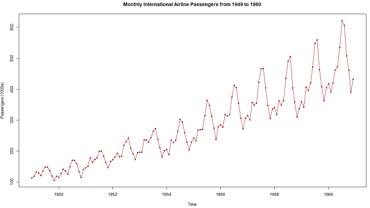
Figure 2.
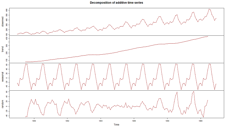
The decomposition model considered is an additive model with the form
Yt = Tt + Ct + St + It
where Yt is the observed value at time t,
Tt is the trend component value at time t,
Ct is the cycle component value at time t,
St is the seasonality component value at time t,
It is the irregularity component value at time t.
We can observe from the chart of the time series data, as shown in Figure 1 above, an overall increase in the monthly total international airline passengers overtime and some periodic spikes every year. By decomposing the time series, we can have a better view of these patterns. Figure 2 shows the time series decomposition of the airline passengers data using an additive model. The second sub-chart shows the trend-cycle component of the time series. We can observe that there is indeed a steady increase in the monthly total international airline passengers but with no visible cyclic pattern. Seasonality is also observed in the third sub-chart as we can see similar periodic patterns every year indicating seasonality. Every March, there is a moderate spike and would slightly go down in the following months but would show a big spike in the total airline passengers by July and August. Then it would suddenly go down until November and slightly increase again by December. These patterns can be observed happening every year, hence an obvious indication of seasonality. The irregular or residual component, as shown on the bottom sub-chart, also shows some interesting behavior having high variability in the early years and the latter part of the time series.
Click here to know more about the advanced analytics and data science services by N-PAX. For consultations, you can contact us at info@n-pax.com
Recent Blogs